
Recent posts
#11
Geometry, Material & Navigation / Re: Is navigator order suppose...
Last post by mwj12 - Dec 10, 2025, 05:58 PMOK, but if that's the case, it sounds like if I list the bowtie first, then a primary photon will propagate correctly, but back-scatter from the CBCT detector can never propagate correctly. A back-scattered photon should encounter the phantom first, but if the bowtie is constructed first in the .py script, it will encounter the bowtie first, based on what you are saying.
#12
Geometry, Material & Navigation / Re: The x'-y'-z' origin for vo...
Last post by mwj12 - Dec 10, 2025, 05:50 PMThanks, but to be clear, If I want the center of the voxel grid at world coordinates (tx,ty,tz), then,
Code Select
set_position(tx, ty, tz, 'mm') is the right thing to do? #13
Output Data / Re: Improving histogramming ef...
Last post by didier.benoit - Dec 10, 2025, 01:41 PMThanks for the suggestion — you are correct that the code in v1.3 performs two atomic additions when a scattered detection occurs, and that this can be reduced to a single atomic operation. However, in GGEMS v1.3 the two histogram buffers have different semantics:
- histogram stores all detected events (primary + scatter)
- scatter_histogram stores only scattered events
Therefore, even when an event is scattered, the total histogram must still increment, because it represents the full projection image as detected by the system. The two buffers are not redundant; they encode different physical quantities. The alternative implementation you propose (only incrementing one buffer and reconstructing the total histogram afterwards) is technically possible, but it would move part of the tally logic outside the kernel and slightly change the meaning of the intermediate results produced during a run. For the design of v1.3, we kept the histogram semantics explicit inside the kernel, even at the cost of an additional atomic operation.
#14
Output Data / Re: CBCT simulation output ex...
Last post by didier.benoit - Dec 10, 2025, 01:34 PMWhat you are observing is expected behaviour in GGEMS v1.3. The geometry engine in this version does not support hierarchical or nested mesh volumes (no mother/daughter relationship, no enclosure detection, and no overlap resolution). All meshed objects are treated as independent top-level volumes. During transport, GGEMS v1.3 evaluates navigators in a flat list, and the first navigator that intercepts the ray "wins". If a mesh volume is fully enclosed inside another mesh volume, the outer volume will always intercept the particle before the inner one. As a result, the enclosed mesh is never queried, and it effectively disappears from the simulation.
This explains why:
- When the cylindrical soil is fully inside the centrifuge tube, it does not appear in the projection.
- When you move it slightly so that it protrudes outside the tube, it becomes visible again (because it can now be the first object intersected by the ray).
This limitation is inherent to the v1.3 geometry system and cannot be resolved by STL positioning alone.
The upcoming GGEMS v2 introduces a unified geometry framework with proper hierarchy and overlap handling, in which nested or enclosed meshes will be correctly represented.
#15
Geometry, Material & Navigation / Re: Is navigator order suppose...
Last post by didier.benoit - Dec 10, 2025, 01:30 PMIn GGEMS v1.3, the order in which navigators are defined does affect the simulation, especially when volumes overlap or one volume lies inside the bounding box of another. This is expected behaviour for the v1.3 geometry system.
The reason is that v1.3 does not implement a hierarchical geometry (no mother/daughter volumes) and does not perform overlap resolution. All navigators are stored in a simple linear list, and during particle transport the engine queries them in the order they were created.
The first navigator that reports an intersection is taken as the active geometry for that step.
As a consequence:
- If a meshed navigator (bowtie, collimator) is defined before the voxelized phantom, the meshed object is encountered first, and the projection looks correct.
-If the voxelized phantom is defined before the meshed navigators, the phantom intercepts the particles earlier, effectively masking the mesh geometry and producing artifacts.
So the results you observe (Mesh→Vox giving correct projections, Vox→Mesh producing strong artifacts) are consistent with the internal design of v1.3.
This behaviour will be redesigned in GGEMS v2, which will introduce a unified geometry system with proper hierarchy and overlap handling, so that navigator ordering will no longer affect physics results.
#16
Geometry, Material & Navigation / Re: Creating geometry componen...
Last post by didier.benoit - Dec 10, 2025, 01:25 PMIn GGEMS v1.3, Python is intentionally minimalistic. It does not manage the geometry, nor introspect lists or containers. Its only role is to create a few objects and pass them to the C++ engine, which performs all simulation work.Therefore, components must be exposed as simple top-level variables so that the C++ core can register them.
#17
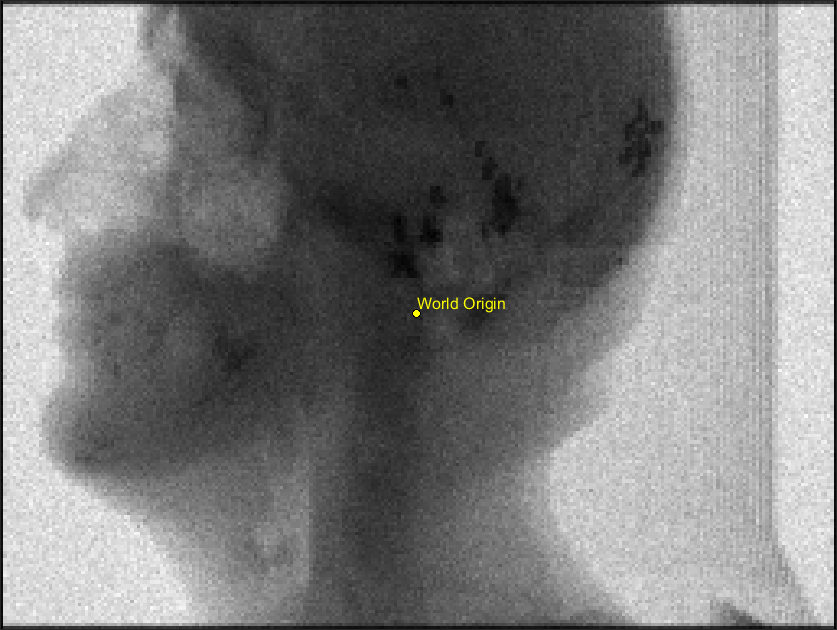
Geometry, Material & Navigation / Re: The x'-y'-z' origin for vo...
Last post by didier.benoit - Dec 10, 2025, 01:19 PMThanks for the detailed observation — this is indeed a point where the GGEMS v1.3 implementation behaves differently from what the documentation suggests.
In the voxelized geometry module of v1.3, the voxel grid is internally indexed from a corner, but when the phantom is constructed and positioned in the world, the engine applies a transformation that implicitly recentres the volume around its geometric centre.
As a result, calling:
phantom.set_position(0.0, 0.0, 0.0, "mm");
places the centre of the phantom at the world origin, not the corner of the voxel grid.This behaviour is consistent with what you are seeing, and it is expected for the current v1.3 implementation. This centring step was historically introduced to simplify rotations and transformations, but it does create an inconsistency between the documented "corner origin" and the effective placement of the object in world coordinates.
We will address this properly in GGEMS v2, where the coordinate conventions will be made fully explicit and consistent (local origin, centre, positioning, and rotations). The goal is to remove this ambiguity entirely and adopt a single, predictable convention across the whole geometry system.
#18
Geometry, Material & Navigation / Is navigator order supposed to...
Last post by mwj12 - Dec 08, 2025, 04:27 AMI find that I get substantially different simulation results depending on the order in which navigators are defined. In the attached file MeshVox.py, I define meshed navigators first (for a CBCT bowtie and collimator) and a voxelized navigator second (the phantom). This leads to the simulated projection image shown in the attached MeshVox.png, which is how the result should look. However, if I interchange the order of the meshed and voxelized navigators (see VoxMesh.py) then the result exhibits a strong artifact (see VoxMesh.png).
Is this expected behavior? If so, what are the precise rules for how the ordering determines navigation geometry?
Is this expected behavior? If so, what are the precise rules for how the ordering determines navigation geometry?
#19
Geometry, Material & Navigation / The x'-y'-z' origin for voxeli...
Last post by mwj12 - Dec 07, 2025, 07:15 PMIn the documentation for voxelized navigators in v1.3, the diagram shows the local coordinate system (x',y',z') of the voxel volume to have its origin at one corner of the voxel grid (I'm not sure if that's supposed to be the center of the first voxel or the voxel's outermost corner...)
However, all of the behavior I'm seeing suggests that the origin is instead at the center of the voxel grid. In particular, when I set up a phantom with the following
If the (x',y',z') origin is at the corner of the voxel grid, shouldn't
However, all of the behavior I'm seeing suggests that the origin is instead at the center of the voxel grid. In particular, when I set up a phantom with the following
Code Select
phantom = GGEMSVoxelizedPhantom('anthropomorphic')
phantom.set_phantom('data/anthropomorphic.mhd', 'data/range_anthropomorphic.txt')
phantom.set_rotation(0.0, 0.0, 0.0, 'deg')
phantom.set_position(0.0, 0.0, 0.0, 'mm')
the simulation results I'm getting are consistent with a phantom centered at the world origin. If the (x',y',z') origin is at the corner of the voxel grid, shouldn't
Code Select
set_position(0.0, 0.0, 0.0, 'mm') put the corner of the voxel grid at the world origin, rather than the phantom's center? #20
Output Data / Improving histogramming effici...
Last post by mwj12 - Dec 06, 2025, 01:48 AMThis section of kernel code in TrackThroughGGEMSSolidBox.cl looks like it could be made more efficient (this is v1.3). Specifically, if we are storing scatter separately, it doesn't make sense to increment both histogram arrays (&histogram and &scatter_histogram) when a scattered detection occurs.
Instead,one can increment just one of the histogram counters, e.g.,
This would eliminate an atomic add. One might still want the final &histogram to be a combined tally of both primary and scattered events, but that can be done trivially by adding the two histograms together at the end of the simulation.
Code Select
 atomic_add(&histogram[voxel_id.x + voxel_id.y * virtual_element_number.x], 1);

  // Storing scatter
  if (scatter_histogram) {
     if (primary_particle->scatter_[global_id] == TRUE) atomic_add(&scatter_histogram[voxel_id.x + voxel_id.y * virtual_element_number.x], 1);
  }
Instead,one can increment just one of the histogram counters, e.g.,
Code Select
const unsigned int idx =
    (unsigned int)voxel_id.x +
    (unsigned int)voxel_id.y * (unsigned int)virtual_element_number.x;

if (scatter_histogram && primary_particle->scatter_[global_id]) {
    atomic_add(&scatter_histogram[idx], 1u);
} else {
    atomic_add(&histogram[idx], 1u);
}
This would eliminate an atomic add. One might still want the final &histogram to be a combined tally of both primary and scattered events, but that can be done trivially by adding the two histograms together at the end of the simulation.